Back to the small box
At the end of the prologue, we left the Vision Transformer’s figure1 with one corner still to explore. In the top left sits a small box that holds the model’s answer: bird, ball, car. A photograph goes in at the bottom, cut into squares, and a single word comes out at the top.
Before following how that word became a sentence, it is worth opening the box itself. What does the model actually do with a photograph? What does it see, and what can it say about what it sees?
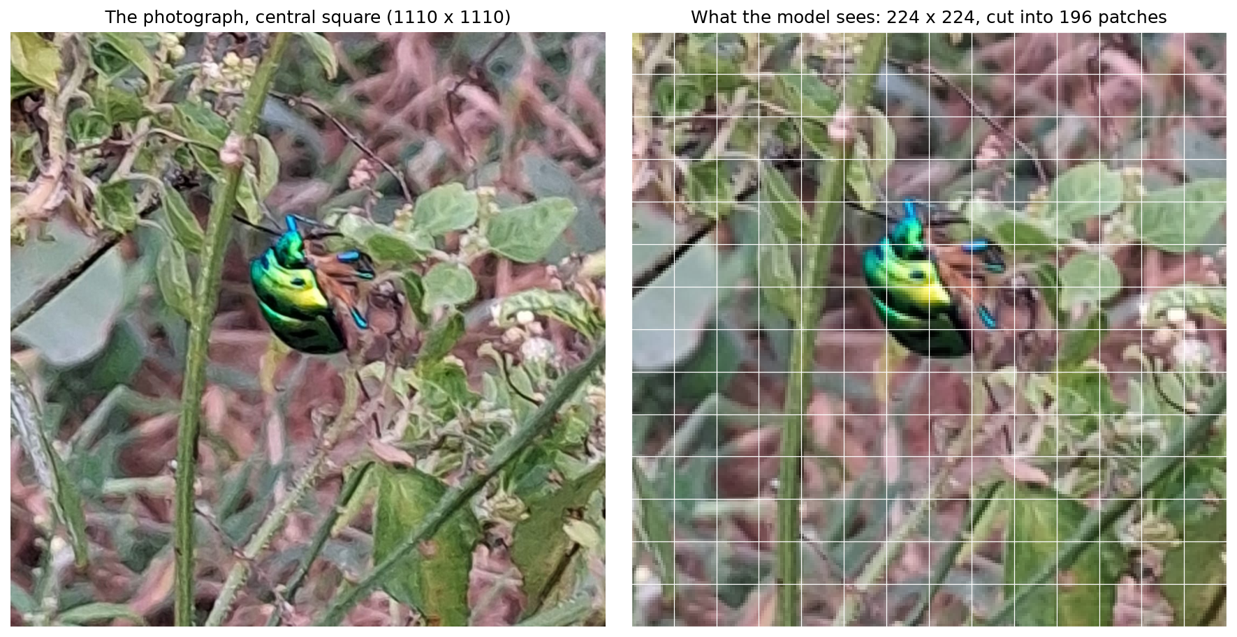
Left: the photograph, 1513 × 1110 pixels. Right: what the model keeps, a 224 × 224 square from the centre, cut into 196 patches of 16 × 16 pixels.
To find out, I gave a Vision Transformer two photographs of my own. One is a beetle, bright green, resting among leaves. The other is a squirrel in a tree, in the middle of a meal. The model is the one from the paper, ViT-B/16, in the version that comes with PyTorch’s torchvision library. Everything in this post ran on an ordinary desktop graphics card, and the notebook is in the companion repository, so you can follow along, or try it with your own photographs.
The beetle and the squirrel had rather different afternoons.
Cutting a photograph into squares
The first thing I did was open the photograph and keep its central square.
from PIL import Image, ImageOps
from torchvision.transforms import functional as F

im = ImageOps.exif_transpose(Image.open("photo-01.jpg")).convert("RGB")
im = F.center_crop(im, min(im.size))
print(im.size)   # (1110, 1110)
Line by line:
Image.openreads the file with Pillow, Python’s usual library for images.- Phones often save a photograph sideways, with a small note inside the file, an EXIF tag, saying which way up it goes.
exif_transposereads that note and turns the picture the right way round. convert("RGB")makes sure every pixel, every dot of the picture, is exactly three numbers: how much red, how much green and how much blue. Each of these three is called a channel.center_cropkeeps the largest square from the middle. The photograph was 1513 × 1110 pixels; the square is 1110 × 1110.
I cut the square so that the two pictures in the figure above line up. The model would have cropped to a square anyway, as the next step shows.
Every trained model expects its input in one particular form, and torchvision keeps that form together with the model:
from torchvision.models import ViT_B_16_Weights

weights = ViT_B_16_Weights.IMAGENET1K_V1
preprocess = weights.transforms()

x = preprocess(im)
print(tuple(x.shape))   # (3, 224, 224)
According to the library’s documentation2, preprocess does four things:
- It resizes the picture so that its shorter side is 256 pixels.
- It keeps a 224 × 224 square from the centre.
- It rescales every pixel value from the range 0–255 to the range 0.0–1.0.
- It normalises each channel: it subtracts an average and divides by a spread (the standard deviation). The averages, 0.485 for red, 0.456 for green and 0.406 for blue, were measured over the ImageNet photographs the model learned from. After this step, the numbers sit around zero, in the same range the model saw during training.
What comes out is a tensor: a block of numbers arranged along several directions, much like a spreadsheet with more than two sides. Its shape, (3, 224, 224), reads as 3 channels, 224 rows and 224 columns. The recipe is older than the Vision Transformer. In 2012, AlexNet rescaled every photograph so that its shorter side was 256 pixels, cut 224 × 224 squares from it, and subtracted the average value of the training images from every pixel3. Its paper describes the network’s input as 150,528 numbers: 3 × 224 × 224, exactly the size of the tensor we have here.
In all, the model receives 224 × 224 = 50,176 pixels. The photograph had about 1.7 million.
Now the step that gives the Vision Transformer its name. The 224 × 224 square is cut into smaller squares, 16 pixels on each side. 224 divided by 16 is 14, so the grid is 14 across and 14 down: 196 squares in all. These are the patches, and the grid on the right of the figure above shows exactly where the cuts fall.
The beetle covers about a dozen of the 196 patches. Everything else is leaves, stems and pale flowers. To the model, every patch is simply 16 × 16 pixels of colour, and none is marked as more important than another. Whatever it concludes about the beetle, it will have to work out from these squares, and from how they relate to one another.
Those 196 squares are all the model will ever know about this photograph.
From squares to tokens
Next, I loaded the model itself.
from torchvision.models import vit_b_16

model = vit_b_16(weights=weights).eval()

x = x.unsqueeze(0)
print(tuple(x.shape))   # (1, 3, 224, 224)
vit_b_16builds the model’s structure, its architecture, andweights=fills it with trained numbers. These numbers are the model’s parameters: 86,567,656 of them, in a file of about 330 MB2. The torchvision team trained these particular weights themselves, from scratch, on ImageNet’s 1,000 categories, using a modified version of the DeiT recipe4. They aren’t the paper’s original weights, which were first trained on much larger collections of images1..eval()puts the model in evaluation mode. Some layers behave differently while a model is being trained, and this switches them to how they behave when it is used.unsqueeze(0)adds one more direction to the front of the tensor. Models are built to take many pictures at once, a batch, and this makes ours a batch of one. The shape now reads 1 picture, 3 channels, 224 rows, 224 columns.
Then I asked the model to show me how it cuts the picture:
import torch

print(model.conv_proj)
# Conv2d(3, 768, kernel_size=(16, 16), stride=(16, 16))

with torch.no_grad():
    patches = model.conv_proj(x)
print(tuple(patches.shape))   # (1, 768, 14, 14)
The cutting is done by a single layer called conv_proj, and it is a convolution. A convolution slides a small grid of learned numbers, a filter (or kernel), across the picture. At every stop, it multiplies the pixels under the filter by the filter’s own numbers and adds everything up into a single number.
Here the filter is 16 × 16 pixels, and it moves 16 pixels at a time. That step size is called the stride. Because the step is as large as the filter, the filter never overlaps itself: it lands on each patch exactly once, 14 × 14 times in all. And there are 768 different filters, so every patch comes out as 768 numbers. That is the shape we see: for 1 picture, 768 numbers for each square of a 14 × 14 grid. (torch.no_grad() tells PyTorch we’re only reading the model, not training it, so it can skip the bookkeeping that training needs.)
The paper describes this step differently: flatten each patch into one long list of numbers, and multiply it by a matrix. Figure 1 calls it a linear projection of flattened patches. A filter that lands on each patch exactly once does the same arithmetic, and the library uses the convolution because it’s one line and fast.
Count the numbers in one patch: 16 × 16 pixels, 3 channels each, 768 in all. The layer turns those 768 raw numbers into 768 learned ones, the patch’s embedding. In ViT-B/16 the sizes in and out happen to match; the larger ViT-L uses 1,024. The cutter itself has 16 × 16 × 3 × 768 filter numbers, plus one extra number for each filter, 590,592 parameters in all:
print(sum(p.numel() for p in model.conv_proj.parameters()))
Next, the grid becomes a line:
tokens = patches.flatten(2).transpose(1, 2)
print(tuple(tokens.shape))   # (1, 196, 768)
flatten(2)joins the 14 × 14 grid into one row of 196, reading the patches left to right and top to bottom, like words on a page.transpose(1, 2)swaps two directions, so that each of the 196 rows holds one patch’s 768 numbers.
Each row is now a token: the same kind of object a language model makes from a word. The photograph has become a sequence of 196 tokens.
Two more pieces complete it:
cls = model.class_token.expand(1, -1, -1)
sequence = torch.cat([cls, tokens], dim=1)
print(tuple(sequence.shape))                      # (1, 197, 768)
print(tuple(model.encoder.pos_embedding.shape))   # (1, 197, 768)
- The class token is one extra token of 768 learned numbers, placed at the front of the line. It holds no part of the picture. As the sequence passes through the model’s layers, this token gathers information from all 196 patches, and at the very end the answer is read from it. The paper borrows the idea from BERT’s class token15.
expandsimply makes one copy of it for each picture in the batch, andtorch.catjoins it to the front, giving 197 tokens. - The position embeddings are 197 more sets of 768 learned numbers, one for each place in the line. Once the grid is flattened, nothing in a token says where its patch came from, and the model’s main mechanism, attention, treats its tokens as a set with no order of its own. Adding a position embedding to each token tells the model where it sits. In
torchvision, the encoder adds them just before the first layer.
Finally, a check that my steps match what the library does on its own:
print(torch.allclose(tokens, model._process_input(x))) # True
_process_input is the library’s own version of the cutting, flattening and swapping (the underscore marks it as internal). True means the three lines above do exactly what the library does.
The photograph is now a sequence of 197 tokens, each a list of 768 numbers. From here on, the model is the Transformer encoder from the prologue, the same kind that reads sentences, and nothing in it is specific to pictures.
The answer
With the photograph turned into 197 tokens, I ran the whole model and asked for its five best guesses.
with torch.no_grad():
    logits = model(x)

probs = logits.softmax(dim=-1)[0]
top = probs.topk(5)
labels = weights.meta["categories"]

for p, i in zip(top.values.tolist(), top.indices.tolist()):
    print(f"{p:6.1%}  {labels[i]}")
 75.3%  leaf beetle
  6.9%  tiger beetle
  2.7%  fly
  2.5%  ground beetle
  0.5%  bee
Line by line:
model(x)runs the whole model on the picture, from the cutting all the way to the answer. This is called a forward pass. The 197 tokens go through the twelve layers of the Transformer encoder1, where every token can look at every other one. At the end, the model takes only the class token, whose 768 numbers have by now gathered information from all 196 patches, and passes it through one last layer, the head. The head turns those 768 numbers into 1,000: one score for each label on the model’s list.- These raw scores are called logits. They can be any size, positive or negative.
softmaxturns them into probabilities: numbers between 0 and 1 that add up to 1 across all 1,000 labels. [0]picks out our one picture from the batch.topk(5)finds the five largest probabilities, and where they sit in the list.weights.meta["categories"]holds the names of the 1,000 labels, in the same order as the scores, so position 300 in the scores matches name 300 in the list.
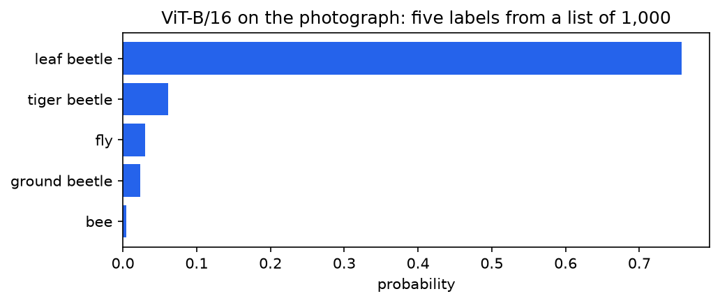
The model’s five best guesses for the beetle, out of a list of 1,000.
The model answered leaf beetle, with 75.3%, and all four of its other guesses are insects. Whether it chose the right family, I’ll leave to someone who knows beetles. It certainly found a beetle, from about a dozen of the 196 patches, surrounded by leaves.
The AlexNet paper noticed the same kind of behaviour in 2012: for a photograph of a leopard, the only other labels its model considered plausible were other kinds of cat3. When a model is right, its second guesses tend to be right in spirit too.
The squirrel
Then I gave the model the second photograph: a squirrel in a tree, eating. Same model, same steps, wrapped in a small function so it can be used again:
def look(im, top_k=5):
    with torch.no_grad():
        p = model(preprocess(im).unsqueeze(0)).softmax(dim=-1)[0]
    t = p.topk(top_k)
    return [(labels[i], v) for v, i in zip(t.values.tolist(), t.indices.tolist())]

im2 = ImageOps.exif_transpose(Image.open("photo-02.jpg")).convert("RGB")
im2 = F.center_crop(im2, min(im2.size))

for name, p in look(im2):
    print(f"{p:6.1%}  {name}")
  9.8%  marmoset
  5.6%  mongoose
  4.5%  boa constrictor
  4.4%  macaque
  4.0%  capuchin
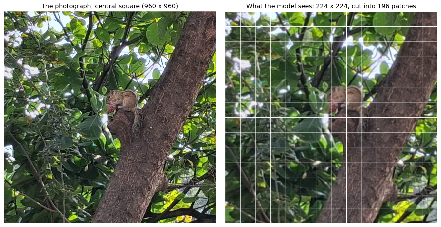
Left: the photograph’s central square, 960 × 960 pixels. Right: what the model keeps, 224 × 224, cut into 196 patches.

The model’s five best guesses for the squirrel. No squirrel among them.
There is no squirrel among the five. And look at the numbers: the best guess, marmoset, has less than 10%, where the beetle’s had 75%. The model is not just wrong here; it is unsure, and the probabilities show it. A confident model puts most of its probability on one label. This one spreads it thinly across many.
What it reached for is telling, though. Three of the five are monkeys, and a mongoose is another small, brown, furry animal. The squirrel sits upright on a branch, holding his food to his mouth with both hands, and a great many photographs of monkeys look exactly like that. The boa constrictor I can only guess at: perhaps the long brown branch curving through the frame. The model doesn’t say why; it only gives the numbers.
The AlexNet paper has a moment very like this one. Among its example photographs is a lemur, listed as Madagascar cat, and AlexNet’s five guesses for it were squirrel monkey, spider monkey, titi, indri and howler monkey3. Thirteen years apart, two different models sent a small animal in a tree to the same corner of the list.
The squirrel, for the record, is not a marmoset.
The list
Why did the beetle go so well, and the squirrel so badly? The answer is in the list itself, so I looked at it.
labels = weights.meta["categories"]

beetles   = [l for l in labels if "beetle" in l]
squirrels = [l for l in labels if "squirrel" in l]

print(len(labels))
print(beetles)
print(squirrels)
1000
['tiger beetle', 'ground beetle', 'long-horned beetle', 'leaf beetle', 'dung beetle', 'rhinoceros beetle']
['fox squirrel', 'squirrel monkey']
These two lines search the 1,000 label names for a word, and keep every name that contains it.
The list comes from the ImageNet challenge (ILSVRC). ImageNet itself holds more than 15 million photographs in about 22,000 categories. The challenge uses a subset of 1,000 of them, with roughly 1,000 photographs each: about 1.2 million training images in all36. Every model trained for that challenge, AlexNet in 2012 and this Vision Transformer alike, learned to answer with one of these 1,000 names, and nothing else.
On beetles, the list is generous: six by name, and a few more that the word search misses, such as ladybug and weevil. On squirrels, it has two entries, and one of them is a monkey. The other, the fox squirrel, lives in North America. The squirrel in my photograph is an Indian palm squirrel, and there is no word for him on the list. So the model did the only thing it can: it chose the names whose pictures looked most like this one.
This is the small box from the Vision Transformer’s figure, bird, ball, car, grown to a thousand words. The eye is good. It found a dozen beetle patches among 196 and named the family. But it can only answer from its list. When the list has the right word, the answer can be very good. When it doesn’t, the model gives you the nearest words it has, and a spread of low probabilities is its way of telling you so.
At your desk
The notebook is in the companion repository: six short cells, each with a note above it. I ran it on Windows with an NVIDIA RTX 3060, a graphics card with 12 GB of memory. The model is small enough that it should also run on an ordinary processor, though I haven’t timed it there. The first run downloads the model’s weights, about 330 MB2.
To try your own photograph, put it in the notebook’s folder and change the file name in the first cell. A good experiment is two photographs: one of something the list knows well, and one of something it doesn’t. The difference in the probabilities is often as interesting as the labels.
Where the list goes next
The Vision Transformer changed how a model looks at a picture: squares instead of a sliding window, tokens instead of pixels, and the same encoder that reads sentences. It didn’t change what the model could say. The answer still came from a fixed list of a thousand words.
That changed in 2021. A model called CLIP learned from 400 million photographs, each paired with the caption someone had written for it on the web7. Instead of a list, it learned to match pictures with sentences, and the small box could hold anything you cared to write. That is where this series goes next: from a list of a thousand words to any sentence, and from there, to a machine that can describe what it sees.
Citations
Alexey Dosovitskiy et al. (2021). An Image is Worth 16x16 Words: Transformers for Image Recognition at Scale. ICLR 2021. https://arxiv.org/abs/2010.11929 ↩︎ ↩︎ ↩︎ ↩︎
PyTorch. torchvision.models.vit_b_16, weights
ViT_B_16_Weights.IMAGENET1K_V1. https://docs.pytorch.org/vision/stable/models/generated/torchvision.models.vit_b_16.html ↩︎ ↩︎ ↩︎Alex Krizhevsky, Ilya Sutskever and Geoffrey E. Hinton (2012). ImageNet Classification with Deep Convolutional Neural Networks. NeurIPS 2012. https://papers.nips.cc/paper/2012/hash/c399862d3b9d6b76c8436e924a68c45b-Abstract.html ↩︎ ↩︎ ↩︎ ↩︎
Hugo Touvron et al. (2021). Training data-efficient image transformers & distillation through attention. ICML 2021. https://arxiv.org/abs/2012.12877 ↩︎
Jacob Devlin et al. (2019). BERT: Pre-training of Deep Bidirectional Transformers for Language Understanding. NAACL 2019. https://arxiv.org/abs/1810.04805 ↩︎
Olga Russakovsky et al. (2015). ImageNet Large Scale Visual Recognition Challenge. International Journal of Computer Vision. https://arxiv.org/abs/1409.0575 ↩︎
Alec Radford et al. (2021). Learning Transferable Visual Models From Natural Language Supervision. ICML 2021. https://arxiv.org/abs/2103.00020 ↩︎